Search among one hundred candidates and keep the winner. In the synthetic experiment below, the winning score averages 88.1 across repetitions of that process. A fresh test of each selected candidate averages 75.6.
That gap could suggest a failed replication or a dishonest report. Neither is necessary here. Every candidate was evaluated under the same rules. The problem was that we remembered only the best first result.
Success is evidence, but the process that makes success visible is part of that evidence. A leaderboard, a collection of surviving companies, and a shelf of famous records are all filtered views. Reading the visible outcome as a transparent measure of underlying quality asks it to do more work than it can support.
In the first essay, I argued that a statistical description of luck needs a declared predictive reference and a boundary around control. Here I examine what happens when the reference is built from winners, or when winning changes the process itself.
A winner can be better and overrated
Consider a synthetic population of candidates. Each has a stable mean performance $\theta_j$, and its first measured score contains occasion-specific variation:
$$\theta_j\sim N(70,4^2),\qquad Y_j=\theta_j+\varepsilon_j,\qquad\varepsilon_j\sim N(0,6^2).$$All latent means and errors are independent. A fresh measurement uses the same $\theta_j$ and a new independent error. The units are an invented continuous score; this is not a model fitted to people’s talent or bounded accuracy percentages.
The joint normal model gives an exact conditional expectation:
$$\mathbb E[\theta_j\mid Y_j=y]=70+\lambda(y-70),\qquad\lambda=\frac{4^2}{4^2+6^2}=\frac4{13}.$$One way to derive it is to note that $\operatorname{Cov}(\theta,Y)=16$ and $\operatorname{Var}(Y)=52$, then use the conditional mean of a bivariate normal. The same expression is the expected fresh score. A first observation of 88 predicts a repeat mean of approximately 75.54, not 88.
Regression toward the population mean follows from the independent repeat design. The candidate has not become less capable; the first score still supplies evidence, with a posterior mean above 70.
I simulated 20,000 independent selection experiments for each candidate-pool size. In every experiment, the candidate with the largest first score was selected, and received a fresh measurement.
| Candidates considered | Mean winning first score | Mean selected latent performance | Mean fresh score |
|---|---|---|---|
| 1 | 69.99 | 70.02 | 70.07 |
| 5 | 78.36 | 72.56 | 72.54 |
| 20 | 83.45 | 74.13 | 74.12 |
| 100 | 88.11 | 75.60 | 75.64 |
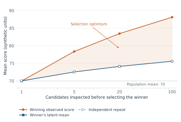
Synthetic results, seed 20261005. Searching more candidates finds stronger candidates while also selecting more favorable measurement noise.
Searching improves the selected latent mean. The winning observation overstates the gain because selection also finds favorable occasion noise.
For independent candidates, $\Pr(\max_jY_j\le t)=F(t)^m$. Increasing $m$ makes an impressive maximum more likely even without changing the candidate distribution. Under this particular Gaussian model,
$$\mathbb E[Y_{j^*}-\theta_{j^*}]=(1-\lambda)\mathbb E[Y_{j^*}-70].$$That identity follows by conditioning on all first scores and using the conditional mean above; $j^*$ is the selected index. It describes average selection optimism. It does not tell us the fraction of one winner’s achievement caused by luck. A different dependence structure, noise level, or candidate population changes the answer.
A population percentage answers a different question
The refusal to divide one achievement into earned and accidental pieces should not obscure a legitimate population estimand: how much of the variation between measured units is reproducible? Reliability theory asks this question directly. Shrout and Fleiss (1979) distinguish forms of the intraclass correlation according to the measurement design and intended application.
For independent repeated measurements under the model above,
$$Y_{ir}=\mu+B_i+\varepsilon_{ir},\qquad \operatorname{Var}(Y_{ir})=\sigma_B^2+\sigma_\varepsilon^2,\qquad \operatorname{Cov}(Y_{i1},Y_{i2})=\sigma_B^2.$$Here B is a persistent unit difference and the errors are independent across occasions and units, with zero conditional means. The correlation between two measurements of the same randomly sampled unit is
$$\mathrm{ICC}=\frac{\sigma_B^2}{\sigma_B^2+\sigma_\varepsilon^2}.$$In our stipulated candidate population, this is 16/52, or 30.77%. For an average of five independent measurements, the corresponding reliability is 16/(16+36/5), or 68.97%. These are shares of measurement variance in this population, not shares of any candidate’s score. Repeat observations can estimate the components: covariance between occasions estimates the persistent component, while half the variance of paired differences estimates occasion noise. In a balanced Gaussian study, the usual within-unit and between-unit mean squares give the same decomposition.
The interpretation is substantial but specific. Persistent differences can include training, resources, stable evaluator bias, or other enduring conditions alongside ability. Calling the numerator “skill” needs evidence about what persists. Shared occasion shocks require an additional component. Changing the population’s range or the number of averaged measurements changes reliability. A narrower population of finalists need not have the ICC of the original candidate pool.
This is the useful distinction: an individual counterfactual asks what would have happened to this unit under a different process; a population variance component asks what differences reproduce under the specified measurement design. We can estimate the latter without pretending to have solved the former.
The record of attempts belongs in the result
In ML, candidates may be hyperparameters, prompts, checkpoints, memory policies, or evaluation rubrics. If each is tested and the highest observed score is reported, the search procedure has selected favorable evaluation variation along with any real improvement.
Cawley and Talbot’s analysis of model selection shows why optimization can overfit a noisy selection criterion. Its practical implication here is to evaluate the selection procedure, with a test set preserved from that search or an appropriate nested design. Repeatedly returning to the supposedly independent test set makes it part of the search again.
Candidate errors are often correlated because all candidates share examples or infrastructure. Our independent Gaussian experiment therefore supplies an illustration, not a correction factor for a real leaderboard. Dependence can change the benefit of search and its optimism. Keeping failed attempts and the selection rule is necessary to investigate that change.
Gelman and Carlin’s design analysis adds another caution: when estimates are noisy relative to plausible effects, selecting statistically significant results can exaggerate magnitude and can sometimes select the wrong sign. Their Type M and Type S questions concern repeated sampling under assumed effect sizes. A large observed winner is a poor substitute for external information about those sizes.
An evaluation should preserve both the opportunity to find an impressive result and evidence that remained untouched by that search.
Survivors are a selected population
Imagine two independent standard normal quantities, $S$ and $U$, and an inclusion rule $S+U>2$. We might call them persistent capacity and favorable circumstance, but those names are interpretations of a toy model. Before selection their correlation is zero. Among selected cases, a lower $S$ generally needs a higher $U$ to cross the threshold.
In 200,000 simulated cases, the full-population correlation was approximately −0.001; among the 15,684 included cases, it was −0.733. Selection created a strong association where none existed in the generating population.
This is a collider mechanism: inclusion depends jointly on two inputs. It explains how studying only successful cases can distort relationships between their characteristics. It does not establish that successful people with one attribute lack another. The threshold and distribution were chosen to demonstrate a possibility, not estimated from human histories.
Jerker Denrell’s work on undersampling failure examines a related learning problem: practices associated with visible survivors can appear more effective than they are across all attempts. The value of a strategy must be assessed over its attempts, including failures absent from the visible record.
The absent denominator matters. A story about the founder who concentrated everything in one risky idea tells us little about all the people who did the same and disappeared from the record. We also need comparable starting conditions, exposure, and the cost of failure. Otherwise the observed biography is doing the work of an experiment that never occurred.
Early outcomes can change later probabilities
In the selection experiment, the first occasion’s favorable variation is not carried into an independent repeat. The new measurement still contains new variation. Some processes instead preserve an early advantage by changing future opportunity.
Take two alternatives, A and B, initially assigned weights one and one. Select an alternative with probability proportional to its current weight, then add one to the selected weight. After $a$ selections of A and $b$ of B,
$$\Pr(\text{next is A}\mid a,b)=\frac{1+a}{2+a+b}.$$This Pólya urn is a minimal reinforcement model. Both alternatives begin symmetrically. There is no built-in quality difference. Yet an early success changes later probabilities.
The mathematics also reveals a limit to our interpretation. For an ordered sequence with $a$ A selections and $b$ B selections, its probability is
$$\frac{B(1+a,1+b)}{B(1,1)}.$$Exactly the same sequence probability results if we first draw a fixed $P\sim\operatorname{Beta}(1,1)$ and then make independent Bernoulli selections conditional on $P$. An observed sequence alone cannot distinguish this urn’s feedback mechanism from that latent-propensity mixture. Their predictive distributions agree even though their causal stories differ.
In the urn interpretation, the long-run A share has a uniform distribution on $[0,1]$. For independent fair selections, it converges to one half. With 500 selections across 20,000 worlds, the simulated share standard deviations were 0.2894 and 0.0224, respectively. The urn simulation uses the exact beta-binomial representation above, rather than iterating each draw.
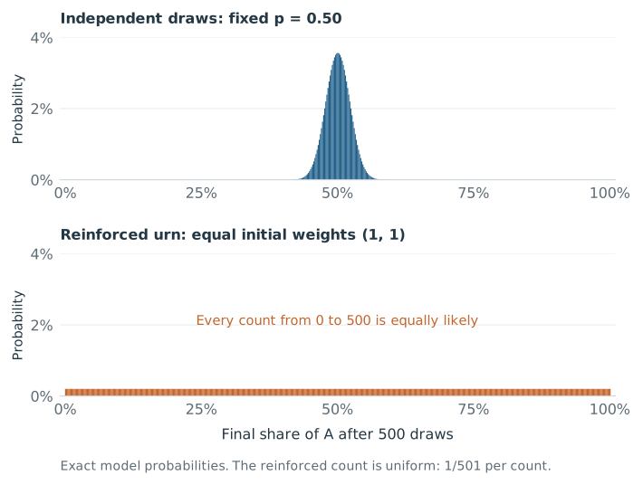
Exact model probabilities for 500 draws. This contrast illustrates persistence of early variation; it does not identify reinforcement from an observed market distribution.
After A wins the first draw, its expected final share at draw 500 becomes $(1+499\times2/3)/500=0.6673$. That calculation is a consequence of this urn’s rules. It is not a measured advantage enjoyed by an actual artist, company, or model.
An intervention reveals why the two causal stories matter. Force the first selection to be A, rather than observing that A happened to win. In the urn, also apply its ordinary weight update: future draws then begin at weights (2,1), giving an expected final A share of 0.6673. In the fixed-propensity model, forcing the first selection supplies no information about the previously drawn P and does not change it. The expected final share is instead $(1+499\times1/2)/500=0.501$.
Observing the first win and forcing it are different operations. The observable histories agree under the two unmodified models; their responses to this specified intervention do not. To infer reinforcement in a real process, we need evidence that bears on the mechanism, rather than only a distribution with unequal winners.
What experimental evidence adds
The Music Lab experiment by Salganik, Dodds, and Watts is valuable because it created parallel cultural markets rather than merely describing an existing ranking. Participants encountered unfamiliar songs under different social-information conditions. Across its experiments, stronger social influence increased inequality and made success less predictable across parallel worlds. Its independent-choice condition supplies a behavioral reference for appeal, not an objective definition of artistic worth. The setting also cannot establish the magnitude of feedback in today’s streaming platforms.
Bol, de Vaan, and van de Rijt’s study of science funding uses a funding cutoff to compare applicants near the threshold. It provides evidence of cumulative funding advantage in that local setting, including later participation differences. The causal interpretation depends on the regression-discontinuity design’s assumptions. It is neither a general percentage of scientific success due to luck nor evidence that all winners and nonwinners were identical.
Each study connects a mechanism to a design and population that can test it. Their strength comes from that specificity.
The simulation Talent versus Luck by Pluchino, Biondo, and Rapisarda asks a different question: what outcomes can follow from stipulated encounters and compounding rewards? It is useful as a generative thought experiment. Its talent distribution, opportunities, and capital update rules are assumptions. A simulated concentration of wealth cannot validate those assumptions or estimate luck’s contribution to actual wealth.
Selection, exposure, and reinforcement must therefore be investigated separately, with evidence appropriate to each. A generative model can make a mechanism explicit without showing that it generated the world we observed.
A conclusion that does not erase ability
Selection finds stronger candidates and favorable noise together. Reliability estimates how much variation reproduces across occasions. Experimental changes to exposure can distinguish mechanisms that ordinary histories leave observationally equivalent. These are complementary questions; together they make success more informative than a winning score alone.
An impressive result deserves an account of how it became visible: preserve the attempt history, state the selection rule, seek independent repetition, and investigate the mechanism that shaped later exposure. Those are also the ingredients needed to evaluate an AI system without mistaking its most fortunate run for its expected behavior.
The study package supplies the code, full numerical results, and source and assumption notes. Every simulated quantity in this essay is synthetic; the cited studies retain their own populations and identification limits.