Fifteen successes in twenty attempts. Before knowing anything else, it is tempting to admire the person who achieved them. After learning that the usual success rate is one half, we may begin to speak of good fortune. After learning that it is seven tenths, the same record seems considerably less exceptional.
Nothing about the observed count has changed. What changed was the story we were prepared to tell before seeing it.
That is where a statistical account of luck has to begin. An outcome does not carry its own probability distribution. We supply a population, an information set, a model, and a judgment about which outcomes matter. If those choices remain hidden, the word luck can make an explanation sound precise while leaving its most important commitments unspecified.
This is the first of three essays. I want to find a useful statistical representation of luck, test how selection and accumulated advantage distort it, and then ask what it should change in the evaluation of machine learning and AI systems. The aim is a defensible way of reasoning, rather than a number that divides a life into earned and unearned portions.
The reference-class problem
The choice has an established name: the reference-class problem. One unit belongs to several populations, each potentially supporting a different probability. In Venn’s The Logic of Chance, Chapter IX, the problem appears through a person’s membership in overlapping classes. Hájek’s analysis examines Reichenbach’s proposal to use the narrowest class with reliable statistics and the difficulties it leaves: relevant classes need not be nested, and reliability needs justification.
For a prediction, choose comparable mechanisms and a population relevant to the decision, then test sensitivity to defensible alternatives. Declaring the comparison in advance protects it from hindsight. Its relevance still needs an argument. A token-matched model baseline, human performance, and the process an agent would replace answer different questions even when they use the same score.
A word doing several different jobs
We use luck for a favorable surprise, for circumstances outside someone’s control, and for the consequences of taking a risk. Those meanings overlap, but they are not equivalent.
A person may inherit reliable access to education. That advantage can be highly predictable from their circumstances and still lie outside their control. A system may deliver an unexpectedly good answer because its evaluation omitted an easy subgroup. That surprise may reflect a flawed model of the experiment. A careful decision may have a bad outcome without having been a bad decision.
Frank Knight’s discussion of risk and uncertainty is useful here: a probability calculation presupposes that we can give a defensible account of the relevant possibilities. His distinction cautions against treating a unique, poorly understood situation like a familiar repeated gamble. In this series I will still express uncertain beliefs with probabilities. That is a contemporary modeling choice, accompanied by Knight’s warning about their warrant.
There is also an ethical question that probability does not settle. The opening of Thomas Nagel’s “Moral Luck” places moral assessment in tension with consequences beyond the agent’s control. I take that as a boundary for this series: describing the distribution of consequences cannot, by itself, decide what a person deserves.
Contemporary accounts add another distinction. Pritchard’s modal account asks how easily an event could have failed under nearby alternatives with relevant initial conditions fixed. Modal closeness concerns similarity; it is not itself a probability. Riggs defends a control account against the modal approach. These are competing accounts, rather than two interchangeable definitions.
For an applied investigation, I will ask three related questions: how unexpected was the result under a justified reference; how fragile is it under specified, credible perturbations; and what feasible actions could change it? A perturbation test makes the second question concrete. Calling its failure frequency a probability requires an explicit sampling distribution over perturbations, beyond a judgment that alternatives are nearby.
To keep those questions visible, consider an outcome generated by
$$Y=g(A,X,U).$$Here $A$ denotes a specified action, $X$ the circumstances we choose to represent, and $U$ the remaining inputs. Calling all of $U$ “luck” would be premature. It may include unmeasured ability, an instrument’s error, an omitted institutional constraint, or a genuinely unpredictable event. Even the boundary between $A$ and $X$ depends on the actor and time horizon: a deployment team can change an evaluation protocol this month, but cannot change which users existed last year.
This representation becomes useful when we specify the processes and interventions it is meant to describe.
Surprise and control are two different questions
A favorable deviation from a forecast supplies evidence about surprise. Practical control concerns which actions and circumstances the actor could change. I will keep the two questions separate: How favorable and unexpected was the outcome under the declared prediction? And which consequential circumstances were beyond this actor’s practical control? Their answers may inform an account of luck, but neither supplies the other.
A well-resourced starting position can be predictable yet beyond the recipient’s control. A team’s deliberate improvement can surprise an observer whose forecast omitted the changed procedure. In the first case, little predictive surprise does not erase good fortune. In the second, surprise does not establish it. These classifications depend on the actor, the feasible actions, and the time horizon; control is often partial rather than binary.
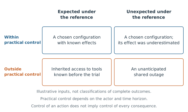
Hypothetical sources of variation, not causal classifications of complete outcomes. Prediction concerns an information set; practical control concerns an actor and a time horizon. Many real cases have mixed control.
For the statistical part, declare the outcome and the prediction before observing the result. For the control part, describe the process and seek evidence about its mechanisms. I use good or bad luck for favorable or unfavorable contingencies beyond practical control, while treating the quantities below as descriptions of the prediction. This working usage does not exhaust the philosophical meanings of luck.
Measuring the predictive excess
Let $I_0$ be the information available before observation and $M$ the modeling assumptions. First declare the predictive distribution
$$Y\mid A,I_0,M \sim F_0.$$If larger values are preferable and the expectation exists, an elementary descriptive quantity is
$$D=y-\mathbb E[Y\mid A,I_0,M].$$Call $D$ the predictive excess. It answers how far the result exceeded its declared expectation, in the outcome’s units. A standardized version divides by the predictive standard deviation when that quantity is finite and nonzero. Neither quantity is a causal share of success, and a positive excess is not automatically good luck. Changing the model can change both.
A percentile answers a different question. For a discrete outcome, I use the mid-distribution rank
$$R(y)=\Pr(Y\lt y\mid A,I_0,M)+\tfrac12\Pr(Y=y\mid A,I_0,M).$$The half-weight handles ties symmetrically; the resulting discrete ranks are not exactly uniform. An upper-tail probability $\Pr(Y\ge y\mid A,I_0,M)$ describes the frequency of outcomes at least this high under the reference. Its direction must be chosen beforehand; causal attribution is a separate estimand.
When higher values are not always better, define the utility or loss first. The same response can be fast and harmful, expensive and accurate, or acceptable to one user and unusable to another. A percentile of a convenient metric is not automatically a percentile of a desirable outcome.
The same record under three references
Suppose the twenty attempts are independent, each with a known success probability $p$. Then $K\sim\operatorname{Binomial}(20,p)$, with mean $20p$ and variance $20p(1-p)$. The upper tail is an exact finite sum:
$$\Pr(K\ge15)=\sum_{k=15}^{20}{20\choose k}p^k(1-p)^{20-k}.$$| Declared success probability | Expected successes | Observed excess at 15 | Probability of 15 or more |
|---|---|---|---|
| 0.50 | 10 | 5 | 2.07% |
| 0.60 | 12 | 3 | 12.56% |
| 0.70 | 14 | 1 | 41.64% |
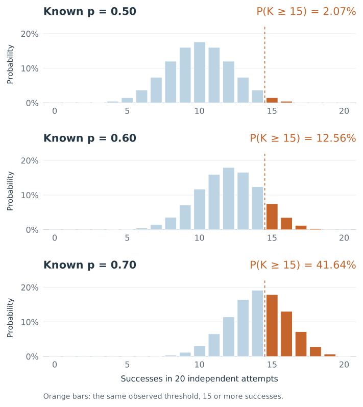
The orange bars show the entire upper-tail event, K ≥ 15. The distributions are stipulated references, not estimates of people’s ability.
The arithmetic is straightforward. Choosing the reference is the difficult part. Should we compare this person with beginners, experienced practitioners, or people with comparable access to tools? Should an AI system be compared with another system under the same budget, or with the process it would replace? Those choices express the question we are asking. They cannot be recovered from the number fifteen alone.
There is a further trap. If we estimate $p$ from these same twenty outcomes and then judge how surprising those outcomes were under the fitted value, we have let the observation rewrite its own expectation. For a prospective assessment, fit on earlier evidence, preserve uncertainty, and freeze the reference before the new outcomes arrive.
The opportunities to notice a result also belong in that reference. Under $p=0.50$, a preselected group has a 2.07% chance of fifteen or more successes. Among one hundred independent groups tested under those same rules, the probability that at least one reaches that threshold is 87.65%:
$$\Pr(\text{at least one qualifying group})=1-(1-0.0206947)^{100}\approx0.8765.$$The count did not become less real. The observation process changed from following one fixed group to searching a hundred. This is the kind of denominator problem emphasized in Diaconis and Mosteller’s study of coincidences: apparent improbability depends on the opportunities and definitions that produced the noticed event. Our numerical example is its own calculation, not a result from their paper. Dependence between groups would change it.
A real comparison that changes with the reference
The public UCBAdmissions table in R records 4,526 applications to six large Berkeley departments in 1973, a subset of the university’s admissions. Bickel, Hammel, and O’Connell’s original study examined how different department mixes complicate aggregate comparisons. I use the published counts for a descriptive reanalysis.
The table records 1,198 admissions among 2,691 applications labeled Male and 557 among 1,835 labeled Female. Those marginal rates are 44.52% and 30.35%. Now ask a different question: what comparison results if both groups are summarized under the same department composition?
For each department d, take its share of all 4,526 applications as the common weight. Apply those weights to each group’s observed departmental admission rates:
$$r_s^{\mathrm{common}}=\sum_d w_dp_{sd},\qquad w_d=\frac{N_{\mathrm{Male},d}+N_{\mathrm{Female},d}}{4526}.$$| Reference composition | Male admission rate | Female admission rate | Female minus male |
|---|---|---|---|
| Each group’s actual department mix | 44.52% | 30.35% | −14.16 percentage points |
| Same pooled department weights | 38.73% | 43.00% | +4.26 percentage points |
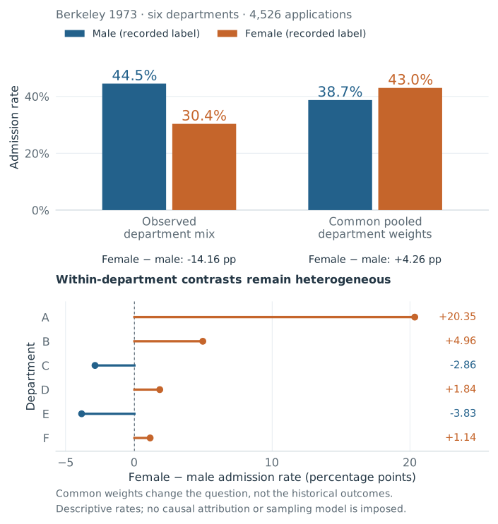
Published 1973 cohort counts from six departments; our pooled-weight standardization. The reference composition changes the descriptive comparison. Department-specific rates remain unchanged.
The direction changes because the questions differ. The marginal rates describe the actual application mixes; standardization compares the groups at a declared common mix. Neither replaces the other automatically. A fairness inquiry must justify the composition it uses, especially when access and prior inequality can influence department choice.
These aggregates contain no individual qualifications or counterfactual admissions decisions. The reversal establishes the importance of the reference; it does not establish the absence of discrimination or measure anyone’s luck. The comparison also varies by department: female rates are higher in A, B, D, and F, and male rates in C and E. The downloadable analysis preserves all twelve aggregate rows and computes both summaries with exact rational arithmetic. Predicting future applicants would require a separate model of comparability across cohorts.
Uncertainty about the probability changes the prediction
Suppose earlier data contained twelve successes in twenty trials. Assume that, conditional on the same fixed but unknown $p$, the earlier and later trials are independent Bernoulli draws. Under a declared uniform prior, $p\sim\operatorname{Beta}(1,1)$, the posterior is $p\mid\text{earlier data}\sim\operatorname{Beta}(13,9)$. For a new batch of twenty trials, integrate over that posterior:
$$\Pr(K=k\mid\text{earlier data})={20\choose k}\frac{B(k+13,20-k+9)}{B(13,9)}.$$The predictive probability of fifteen or more is 19.09%. Comparing it only with the earlier plug-in result, 12.56%, would mix two changes. The posterior mean is $13/22$, slightly below 0.60. We can show the intermediate calculation:
| Treatment of the probability | Mean successes in the new batch | Probability of 15 or more |
|---|---|---|
| Fix p at the earlier proportion, 0.60 | 12.00 | 12.56% |
| Fix p at the posterior mean, 13/22 | 11.82 | 10.95% |
| Integrate over the posterior Beta(13,9) | 11.82 | 19.09% |
The last two rows have the same mean. Their difference isolates the consequence of retaining posterior uncertainty rather than treating its mean as known. Their count variances are 4.83 and 8.83, respectively. More generally, for a posterior mean $m$ and variance $v$, the variance of $n$ new conditional Bernoulli trials is
$$\operatorname{Var}(K\mid\text{earlier data})=nm(1-m)+n(n-1)v.$$The second term expresses uncertainty shared across the predictions. It is not a new physical interaction between trials. Nor does wider variance imply that every chosen tail probability must increase; the increase shown here concerns this particular upper tail.
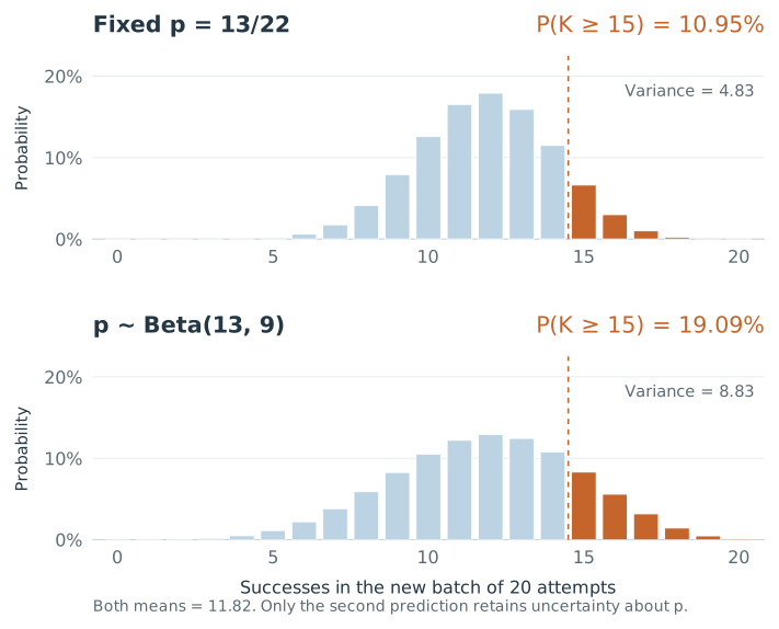
Keep the mean fixed to examine what integrating over an uncertain probability changes. The shaded event is fifteen or more successes in the new batch.
The uniform prior and fixed-probability likelihood are commitments about both batches. Prior sensitivity and changes in the population belong in the assessment of the prediction.
When an environment is shared
Dependence creates another route to wider predictions. Imagine that each batch has its own environment, $P\sim\operatorname{Beta}(2.4,1.6)$, and the twenty trials are independent only conditional on that environment. Their marginal success probability is still $0.60$, but the shared environment induces correlation $0.20$. The count’s variance is
$$\operatorname{Var}(K)=np(1-p)\{1+(n-1)\rho\}=23.04,$$compared with 4.80 under unconditional independence. The beta-binomial mathematics resembles the previous calculation. Its interpretation differs: one model represents uncertainty about a fixed parameter; the other represents changing environments shared by a batch. A wide outcome distribution alone does not tell us which mechanism produced it.
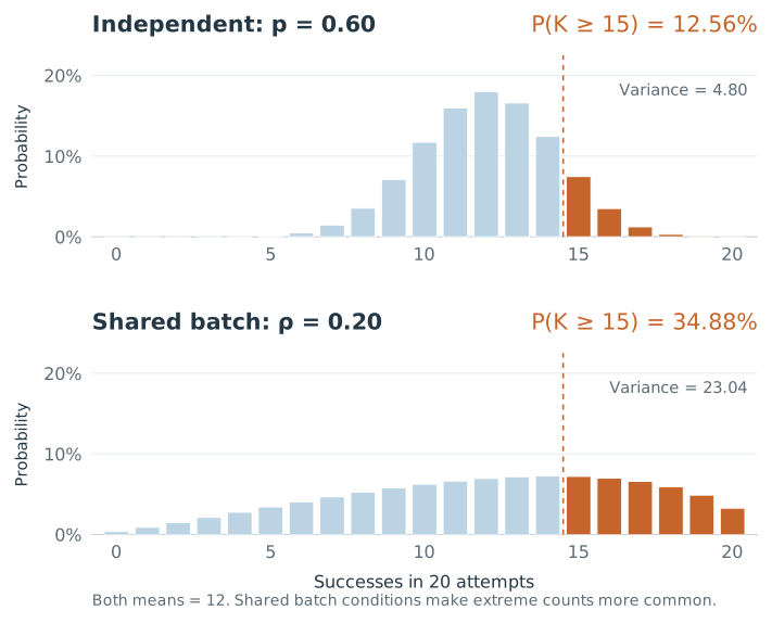
Both models expect twelve successes. Shared exposure changes how much variation survives aggregation. Their count variances are 4.80 and 23.04.
For AI evaluation, imagine responses collected during the same outage, session, or unusually easy batch of prompts. They can share conditions that independent-trial arithmetic ignores. The example shows a mechanism worth investigating; its chosen correlation is not an estimate for any deployed system.
What data would distinguish the mechanisms?
A single count is a poor design for learning about batch variation. Repeated batches change the question. Collect independent batches with recorded environments and multiple trials per batch; keep their identities rather than pooling the successes. A hierarchical model can represent
$$K_b\mid P_b\sim\operatorname{Binomial}(n,P_b),\qquad P_b\sim\operatorname{Beta}(\alpha,\beta),\qquad \mu=\mathbb E[P_b],\quad\tau^2=\operatorname{Var}(P_b).$$For equal batch sizes, its observable count variance is
$$\operatorname{Var}(K_b)=n\mu(1-\mu)+n(n-1)\tau^2.$$The first term is ordinary Bernoulli variation; the second is excess variation shared within a batch. Under this common-beta, conditional-independence model, many independent batches with at least two trials per batch let us estimate both the mean and this excess. A likelihood or Bayesian fit then reports between-batch heterogeneity and uncertainty about the population mean as separate objects. More batches improve our estimate of the mean; they do not make genuinely different environments identical. With one trial per batch, these binary observations contain no within-batch information to identify the extra component.
This design distinguishes the stipulated fixed-p and varying-environment models. Explaining the variation as an outage, task difficulty, or drift requires the corresponding records and design. Crossing the same tasks with several environments helps separate task mix from environmental effects. In AI evaluation, retain task ids, session ids, timestamps, tool versions, and repeat occasions. Those fields determine which hierarchical comparison the data can support.
Turning control into an intervention question
Control becomes operational when we name a feasible change. Let A denote a policy chosen before the outcome, X pre-action conditions, and U external inputs. Treating the equation as a structural model requires a further commitment: the outcome mechanism remains applicable when we set the action differently. Then
$$Y(a)=g(a,X,U),\qquad \Delta=\mathbb E[Y\mid\operatorname{do}(A=a_1)]- \mathbb E[Y\mid\operatorname{do}(A=a_0)].$$The intervention sets an action; conditioning merely selects units that happened to take it. Pearl’s account of structural causal models gives this distinction a formal language. Define the feasible policies, the budget, the outcome, and the population before estimating their contrast. Random assignment supplies evidence about policy effects. Observational comparisons need a defensible account of confounding and overlap in the pre-action conditions.
For an agent, the feasible change might be its retry policy. Evaluate alternative policies on independently sampled environments, with paired runs where a controlled test harness supports them. Inject a specified tool failure and measure whether recovery depends on the policy. That experiment can show which failures an action changes and which environmental variation remains under each action. The third essay develops the replay protocol and its assumptions.
We have now moved from declaring a boundary around control to testing particular consequences of changing actions. It is a causal assessment of a feasible intervention, not a universal partition of a person’s agency.
Check the reference, then learn from it
A declared model becomes credible through checks that match its intended use. For prospective prediction, retain new batches and compare their event frequencies and interval coverage with the forecasts. Examine relevant subgroups and deployment conditions; good average calibration can conceal a poor reference for the decision at hand.
Model diagnosis asks a related question. Gelman, Meng, and Stern’s posterior predictive assessment compares observed discrepancies with replicated data generated under the fitted model. For the batch example, preserve batch identities in those replications and inspect their spread or clustering. Fitting and checking the same data is legitimate for this diagnostic purpose. Its tail area has a different interpretation from a prospective surprise probability or an ordinary uniformly calibrated frequentist p-value.
A failure directs the next investigation: perhaps the task mix changed, the environments vary, or the forecast omitted a known constraint. Better information can explain more variation without changing the circumstances themselves. Predictive improvement and practical control remain separate achievements.
What this account lets us investigate
A statistical account of luck becomes useful when it produces questions that a study can answer. State the population and justify its relevance. Measure the outcome against the prospective prediction. Test how the result changes under credible perturbations. Use repeated observations to learn which variation persists, and interventions to learn what feasible actions change.
These operations supply different estimands. Favorable surprise describes a realization relative to a prediction. Reproducibility describes variation across units and occasions. A policy effect compares intervention distributions. Keeping them distinct allows the investigation to be ambitious without making a tail probability stand in for a causal explanation.
The same outcome can look exceptional under one reference and ordinary under another. The response is to examine why each comparison deserves to guide the decision. That is a substantive task in statistics, with consequences for how we evaluate people, models, and procedures.
The study package contains the calculations, the public admissions table and its provenance, source notes, and the critical-review record. The next essay examines what a selected winner reveals about persistent performance and favorable occasion variation.