An agent finds a supported answer on its third attempt. Its trace shows a useful result, a successful tool call, and a judge’s approval. What did the team improve: the memory policy, the opportunity to try again, or the conditions in which this run happened?
This question becomes practical when a deployment decision rests on the answer. A retry budget is something we can intervene on. A temporary tool outage is something we can record and test. A permissive judge can make a poor policy appear reliable. Calling the remaining uncertainty luck helps only if it leads us to an experiment capable of separating these mechanisms.
Even the amount of evidence needs examination. An evaluation can contain 480 generated answers and still supply only forty independent user histories.
The distinction sounds administrative until it changes the conclusion. In the synthetic experiment below, treating all repeated measurements as independent produces an interval narrow enough to miss the known effect. Respecting the user as a sampling unit produces a wider interval that includes it. Across thousands of repetitions, the narrow interval fails much more often than its label promises.
Thinking carefully about luck changes what we preserve and what we vary: the complete attempt history, the policy we can change, the environments we sample, and the evaluator through which success becomes a score.
The first essay examined reference classes, fragility, and feasible interventions. The second distinguished selected scores from reproducible population variation and examined how advantage persists. Here I assemble a framework from those findings. It is a methodological proposal, with explicit failure conditions, rather than a validated instrument for measuring luck.
Separate the questions before measuring
Surprise, reproducibility, robustness, policy effects, exposure, and deployment risk call for different evidence.
| Question | Statistical object | Evidence needed |
|---|---|---|
| Was this outcome favorable relative to our prediction? | A realized excess, rank, or tail under a frozen predictive distribution | A defensible prospective reference and a defined outcome |
| Which differences reproduce across occasions? | Population variance components and a design-specific reliability coefficient | Repeated units and occasions, with shared shocks represented |
| Does the result survive credible changes? | A policy contrast across specified perturbations | Matched task variants and an explicit perturbation set or sampling law |
| Does changing the policy improve expected outcomes? | A causal contrast such as $\mathbb E[Y(1)-Y(0)]$ | An intervention design or defensible identification assumptions |
| Who receives favorable exposure or starting conditions? | A distribution of access and outcomes across defined groups | Coverage of the opportunity process; causal evidence for mechanism claims |
| Is the policy acceptable under future variation? | Expected loss, tail risk, and specified failure probabilities | Relevant repeated evaluation, uncertainty, and an explicit decision rule |
A single “luck score” would blur these questions. A model may outperform expectation on one occasion while its policy has no average advantage. A policy may improve the average while harming a subgroup. A low average error may coexist with an unacceptable severe-failure rate.
For the causal question, potential outcomes make the comparison explicit. $Y_i(1)$ and $Y_i(0)$ represent what unit $i$ would experience under two defined policies. We usually observe one policy outcome for a given event, not both counterfactuals. Randomized allocation can identify an average contrast under suitable assumptions; it does not identify the missing individual counterpart simply by making the sample large.
Hernán and Robins’ Causal Inference: What If, especially Chapters 1–3, provides the relevant distinctions. Their standard adjustment approach to observational identification requires exchangeability, positivity, and consistency for adequately specified interventions; other identification strategies use different assumptions. In an AI experiment, changing the model, retriever, budget, and rubric together defines a package intervention. It cannot isolate which component helped without additional design.
Nor does a paired benchmark automatically solve the counterfactual problem for a person’s future interaction. We can run both systems on a recorded prompt, but neither may reproduce the user’s behavior under a live conversation. Pairing supports a bounded comparison; transport to deployment requires more assumptions.
A framework in seven commitments
The framework is intentionally a set of commitments rather than an attribution formula. Each step produces something another person can examine.
1. Define the outcome and population. Record the unit, horizon, and direction of preference. An agent’s final answer, complete trajectory, cost, and severe failures are separate outcomes. State the users and tasks the claim concerns.
2. Justify and freeze the reference. Record the baseline, budget, information, predictive assumptions, and estimated uncertainty before confirmation. Compare defensible references and task weights. Advance declaration controls hindsight; relevance requires evidence.
3. Specify feasible interventions and perturbations. State what changes: memory, retries, abstention, or tool behavior. Distinguish policy changes the team can make from environmental variations used to stress the result. Preserve the mechanisms the comparison assumes remain fixed.
4. Design the repetitions. Identify independent environments, reused tasks, and generation repeats. Estimate reproducible and occasion components where the design supports them. A seed sweep measures execution variation conditional on its cases. Bouthillier and colleagues demonstrate why multiple benchmark variance sources deserve separate examination.
5. Preserve development and selection. Save configurations, failures, exclusions, stopping rules, and evaluator revisions. Confirm the selected procedure on evidence untouched by that search, or use a design that accounts for inspection. Cawley and Talbot explain how selection overfits a noisy criterion.
6. Check the instrument and forecasts. Freeze and audit the evaluator. Assess prediction and calibration on relevant held-out outcomes, including important subgroups. Judge disagreement and sampling uncertainty are different evidence about the measurement.
7. State the decision rule. Define the improvement that would matter, unacceptable failures, and the cost of more evidence. Report whether the decision survives changes in reference, dependence, and target conditions.
The following sections turn those records into an evaluation design.
What pass@k says about a fortunate attempt
The distinction between a good output and a reliable procedure appears clearly in code generation. Chen and colleagues’ Evaluating Large Language Models Trained on Code, Section 3 and Appendix A, studies pass@k: success means that at least one of k candidates passes the specified tests. With n ≥ k generated candidates for one problem and c passing candidates, its estimator is
The ratio counts the all-failing subsets among the distinct k-candidate subsets of the recorded pool. It is zero when fewer than k candidates failed. For that fixed pool, the expression is an exact probability under uniform sampling without replacement. Under independent, identically distributed generations for the problem, it is also an unbiased estimate of success in k fresh attempts.
The reason can be seen without a long calculation. Average the indicator that all candidates fail over every k-subset. Each subset contains independent trials with the same failure probability, so each indicator has expectation (1 − p)^k. The subset average therefore has that expectation too; subtracting it from one gives the desired success probability.
Replacing the unknown probability by c/n in the familiar independent-trial formula answers a subtly different question:
Ten candidates with two passing outputs give 0.5333 from the subset estimator and 0.4880 from the plug-in. For new pools with true per-attempt probability 0.20, their expected values are 0.4880 and 0.45056, respectively, by exact finite sums. The nonlinear plug-in is biased downward for k > 1. The calculation notes give the proof and distinguish this sampling bias from the error of an individual estimate.
Compute the estimator separately for each problem, then average according to the declared task weights. Do not transform the benchmark’s average pass@1 into pass@k: two equally weighted problems, one impossible and one certain, average 0.50 at every positive budget. Applying the two-attempt formula to their average probability instead gives 0.75. Difficulty heterogeneity changes the target.
An adaptive agent that reads a failing test before repairing its answer changes the process across attempts. A shared outage or cache may couple them too. The subset formula still describes the recorded pool, but independent fresh attempts are a different target. Evaluate complete adaptive trajectories under their specified policy. The estimator also requires k ≤ n.
Finally, “one correct candidate existed” presumes an evaluator able to recognize it. If the product must choose an answer without hidden tests, report the selected answer’s success rate as well as candidate availability. Include all calls, latency, and cost. A policy that supplies more opportunities for a favorable attempt may be useful, but its benefit belongs to the budgeted procedure.
A held-out label is a claim about the process
A benchmark file can be absent from today’s tuning script and still have influenced the system. Training exposure, copied answer explanations, evaluator development, and repeated prompt refinement are different routes by which a nominal test stops representing unfamiliar evidence.
Oren and colleagues’ contamination test uses canonical-versus-shuffled sequence likelihoods with guarantees under an exchangeability assumption. Its stated limits include uncertainty about real benchmarks’ exchangeability and contamination beyond verbatim exposure. A negative result from such a test is therefore not a certificate of clean generalization. In practice I would retain dataset provenance and exposure notes, separate prompt and judge development from confirmation, and use newly collected target tasks where possible.
There is a second route that does not require anyone to train on the answers. After observing failures, we may redefine the timeout, remove awkward tasks, replace the judge, or change what counts as support. Gelman and Loken’s garden of forking paths explains why data-dependent choices can create a multiplicity problem even when only one final analysis is performed. The engineering consequence is to record those choices as development, then confirm the resulting procedure with evidence that did not guide them.
This does not make every use of existing data illegitimate. A posterior predictive check or exploratory error analysis can use it to ask where a model fails. The misleading step is presenting that same adaptive evidence as an untouched confirmation of the revision it helped produce.
A worked example: repeated users and false precision
Suppose we compare two policies using a paired continuous score difference. There are $n=40$ independently sampled users, $k=3$ tasks per user, and $r=4$ repeated generations per task. That gives 480 differences, $D_{itr}$, generated as
$$D_{itr}=\Delta+U_i+V_{it}+E_{itr},$$where $\Delta=0.02$, $U_i\sim N(0,0.06^2)$, $V_{it}\sim N(0,0.04^2)$, and $E_{itr}\sim N(0,0.04^2)$. All components are independent except that a user’s component is shared across their tasks and a task’s component across its generations.
These are synthetic continuous score units, not observed accuracy differences or probabilities. The model deliberately gives us the true population mean so that we can check interval coverage. It is simple enough to derive the uncertainty exactly:
$$\operatorname{Var}(\bar D)=\frac{\sigma_U^2}{n}+\frac{\sigma_V^2}{nk}+\frac{\sigma_E^2}{nkr}.$$The derivation follows by averaging each independent component. A user component appears twelve times but has coefficient $1/n$ in the grand mean. A task component appears four times with coefficient $1/(nk)$. Only the generation component receives the full $1/(nkr)$ averaging. Substituting the stipulated variances gives a standard deviation of 0.01033 for the grand mean across new panels.
Increasing generations reduces only the final term. More tasks reduce the middle and final terms. More independent users reduce all three. This arithmetic gives a concrete reason why an evaluation can generate more text without adding much information about new-user performance.
For one fixed panel, seed 20261005, the observed mean difference is 0.03481. Average the twelve differences within each user and construct a Student $t$ interval from the forty independent user averages. Under this Gaussian model, those averages are independent and identically normally distributed, so the $t_{39}$ calculation has its usual justification.
| Calculation | Estimated standard error | 95% interval |
|---|---|---|
| Forty independent user averages | 0.01302 | [0.00847, 0.06116] |
| Incorrectly assume 480 independent differences | 0.00439 | [0.02621, 0.04342] |
The second row uses the ordinary row-level standard error and a normal multiplier of 1.96. Its problem is the independence assumption, not a minor difference between $t$ and normal multipliers.
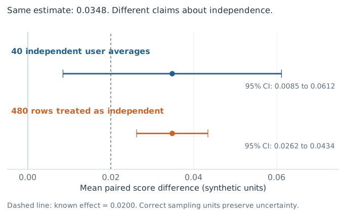
One synthetic panel. The same estimated mean acquires very different apparent precision depending on which observations are treated as independent.
Across 4,000 newly generated panels, the user-level intervals contained the true mean 94.65% of the time. The naive intervals did so 50.28% of the time. The approximate Monte Carlo standard errors of those coverage estimates are 0.36 and 0.79 percentage points. These are simulation frequencies under our stipulated process, not coverage estimates for an actual product.
There is a subtler interpretive issue. Both intervals are above zero in this particular panel, so correcting the dependence does not reverse its directional conclusion. It changes the precision and whether the interval covers the true effect. If a meaningful deployment gain had been declared to be 0.025 score units, the naive lower bound would clear it while the user-level lower bound would not. That threshold is an illustrative decision rule, not one inferred from the data.
The user-level method also has limits. Shared sessions across users, overlapping organizations, or a common evaluator shock may invalidate user independence. With unequal task counts, equal weighting of user means and equal weighting of all responses target different quantities. With nonnormal outcomes and few clusters, the convenient exact justification disappears. And no interval corrects an unrepresentative sample or a rubric that rewards unsupported answers.
A protocol for policies, environments, and replay
Now give the team a concrete intervention. Suppose a support agent can use retrieved memory and can retry a failed tool operation. Test a small factorial design: memory off/on crossed with a retry budget of one/three calls. That gives four specified policies, not four post hoc descriptions of whichever run succeeded. Keep the model, task instructions, and outcome rules fixed so that contrasts isolate these changes and their interaction.
For each independently sampled evaluation environment, run all four policies from the same initial snapshot, restoring state between runs and randomizing policy order. An environment includes the user case, knowledge-base version, account state, and the stipulated process for tool faults. Within this block, pair executions using planned random inputs where the environment permits it. Across blocks, sample new environments. Repeating one favorable snapshot many times measures execution variability conditional on that snapshot; it does not estimate performance across new cases.
| Design layer | Freeze or vary deliberately | Evidence retained |
|---|---|---|
| Policy | Memory off/on × retry budget one/three; fixed stopping and selection rules | Policy hash, complete attempts, selected output, cost and violations |
| Independent environment | New cases and initial states from a declared sampling procedure | Case identity, snapshot hash, sampling weight, shared user or organization |
| Random inputs within a block | Separate tapes for tool faults, simulated responses, and generation when controllable | Event keys, random-input values, actual model outputs and tool results |
| Evaluator | Frozen rubric and judge configuration; blinded labels and balanced answer order | Each judgment, unresolved disagreement, reference evidence and human audit |
Estimate memory’s paired contrast at each retry budget, retry’s contrast at each memory setting, and their interaction. Average over the target distribution of environments, with uncertainty clustered at the level sampled independently. Judge repetitions and extra generations remain measurements within that design. The shared-environment variation from Part I and correlated score differences from Part II tell us why those repetitions should not be counted as new worlds.
Test fragility with a declared perturbation suite
Before confirmation, specify plausible variations: equivalent task phrasings, bounded retrieval degradation, defined delays, or a documented tool-failure pattern. Apply the same variants to every policy and report which contrasts survive. A fixed suite supports sensitivity and worst-case summaries over that suite. Estimating a failure probability requires a sampling law and weights that connect the variations to target conditions. Testing a few convenient perturbations supplies neither a universal robustness guarantee nor a frequency for imagined nearby worlds.
What a seed can preserve
A single seed is not the complete state of an agent’s world. If one policy makes an extra call, it may consume an extra random number; the next draw can then govern a different event in the other branch. Use separate random streams for separate mechanisms and, where meaningful, index environment randomness by a stable event identity rather than by the next position in a global generator. Document the coupling: it must preserve each policy’s marginal environment process, and it can increase or reduce the contrast’s variance. When histories diverge so far that events cannot be matched, acknowledge that pairing limitation rather than forcing two unrelated calls to share a draw.
Hosted generation introduces another boundary. Thinking Machines Lab’s inference experiments show how changing batch size can alter numerical results without changing the individual request. A caller’s sampling seed cannot control every serving condition. Record the returned outputs, model identifiers, request parameters, timestamps, and any available service revision. Report observed reproduction fidelity; do not infer exact reproducibility merely from temperature zero or matching seeds.
Replay the evidence; intervene on a valid environment
For a recorded timeout, preserve the request, arguments, tool version, response or exception, elapsed time, and state before and after the call. Replaying those recorded inputs is useful for verifying the harness. It does not, by itself, reveal what another policy would have done.
An intervention may replace that timeout by a successful response, change the retry rule, or remove an untrusted memory item. Restore a valid initial state, apply the stated intervention, and re-execute downstream decisions over multiple continuations. Reuse a recorded tool response only when its request and relevant state match. If the new policy asks a different question or changes the account, use a stateful sandbox or explicitly specified simulator capable of producing a valid response. Feeding it the old branch’s next response can manufacture a counterfactual that the environment could never produce.
A recent preprint, Shah’s Causal Agent Replay, explores such continuation distributions with synthetic causal validation and mocked tools, providing further reading rather than empirical validation of this protocol.
Rerunning downstream steps also changes downstream randomness unless a defensible coupling holds it fixed. State whether the contrast targets a policy’s total effect over fresh continuations or a more conditional intervention. A simulator can identify contrasts under its mechanisms. It cannot reconstruct the unobserved trajectory of a real user who received a different response. Validate important simulator behavior against held-out interactions, then confirm consequential policy gains in prospective live allocation when appropriate.
Keep the judge from becoming another selected winner
Freeze the judge’s model, prompt, rubric, reference material, and aggregation rule before confirmation. Hide policy labels. Balance the order of paired outputs, retain replicate judgments, and decide in advance how ties and disagreements will be handled. Zheng and colleagues’ judge study documents position and verbosity biases in its settings; repeating a judge can estimate its variability without eliminating its systematic errors.
Prefer executable checks for tool-state changes and verifiable source support where those match the outcome. Audit a blinded sample against independent human review. Keep performance uncertainty, evaluator disagreement, and severe-failure counts visible separately. That leaves the team with something it can act on: a policy contrast, a failure mechanism tested by intervention, and a record of how much of the result survives changes in environment.
Forecasting uncertainty honestly
If a system reports a probability $q$ for a binary event $Y$, the Brier loss is $(q-Y)^2$. With a true event probability $p$,
$$\mathbb E[(q-Y)^2]=p(1-p)+(q-p)^2.$$The first term is irreducible outcome variation under this Bernoulli model. The second penalizes departure from the true probability. Expected loss is uniquely minimized at $q=p$.
That small derivation captures the purpose of a proper scoring rule. Gneiting and Raftery give the broader theory: evaluate predictive distributions with rules that reward honest probabilities in expectation. A rare event occurring once does not make the earlier forecast wrong. Conversely, getting one outcome right does not make an overconfident forecast reliable.
In practice $p$ is unknown. Repeated held-out predictions, uncertainty, and calibration checks are needed; dependence and changing populations complicate them. A language model’s verbal confidence is also not automatically a calibrated event probability. We need a defined event and evidence connecting the reported probability to that event.
What the investigation delivers
The output is a policy contrast under declared conditions, an estimate of which variation reproduces, and evidence about the failures a feasible intervention changes. A population reliability coefficient is a legitimate variance estimand. Calling its persistent component skill, or dividing one person’s achievement into earned and accidental shares, requires a different argument.
The practical conclusion is to let the question determine the design. Use justified references for surprise, repeated occasions for reproducibility, specified perturbations for fragility, and interventions for policy effects. The language of luck is useful when it keeps contingent conditions visible and prompts these investigations.
For an agent team, a fortunate run establishes a possibility worth examining. The deployment decision depends on how often the complete procedure helps the intended users, what it costs, and how it behaves in the environments where it fails.
The study package contains all calculations, synthetic data summaries, figures, source notes, and critical-review decisions.